Note
Click here to download the full example code
Split-half analysis for selecting the number of components
In this example, we will look at how we can use split-half analysis to select the number of PARAFAC components.
The idea of split-half analysis is that we want to find the same underlying patterns if we look at different representative subsets of the same data. To accomplish this, we split the dataset in two equally sized non-overlapping pieces along one mode and fit a PARAFAC model to both pieces. Then, we compare the similarity of the factors in the other, non-split modes.
Generally, we would split the sample mode, but sometimes, it may also make sense to split other modes. For example, if we have a time series and expect the same patterns to be present in two subsequent periods, then we may split the data along the temporal mode instead.
Imports and utilities
import matplotlib.pyplot as plt
import numpy as np
import pandas as pd
from tensorly.decomposition import parafac

import tlviz

rng = np.random.default_rng(0)
To fit PARAFAC models, we need to solve a non-convex optimization problem, possibly with local minima. It is therefore useful to fit several models with the same number of components using many different random initialisations.
def fit_many_parafac(X, num_components, num_inits=10):
    return [
        parafac(
            X,
            num_components,
            n_iter_max=2000,
            tol=1e-8,
            init="random",
            orthogonalise=True,
            linesearch=True,
            random_state=i,
        )
        for i in range(num_inits)
    ]
Creating simulated data
We start with some simulated data, since then, we know exactly how many components there are in the data.
cp_tensor, dataset = tlviz.data.simulated_random_cp_tensor((30, 40, 50), 4, noise_level=0.2, labelled=True)
Splitting the data
We split the data randomly along the second mode
I, J, K = dataset.shape

permutation = rng.permutation(J)
splits = [
    dataset.loc[{"Mode 1": permutation[: J // 2]}],
    dataset.loc[{"Mode 1": permutation[J // 2 :]}],
]
Fitting models to the split data
We split the data randomly along the second mode
models = {}
for rank in [1, 2, 3, 4, 5]:
    print(f"{rank} components")
    models[rank] = []
    for split in splits:
        current_models = fit_many_parafac(split.data, rank)
        current_model = tlviz.multimodel_evaluation.get_model_with_lowest_error(current_models, split)
        models[rank].append(current_model)
1 components
2 components
3 components
4 components
5 components
Computing factor similarity
Now, we compute the similarity between the two splits for the different numbers of components.
However, we cannot compare the second mode (mode=1), since that was the mode we sampled randomly
in. Also, we cannot consider the weights in the factor match score since the weight will also be
affected by the sampling.
split_half_stability = {}
for rank, (cp_1, cp_2) in models.items():
    fms = tlviz.factor_tools.factor_match_score(cp_1, cp_2, consider_weights=False, skip_mode=1)
    split_half_stability[rank] = fms
Plotting the factor similarity
fig, ax = plt.subplots()
ax.plot(split_half_stability.keys(), split_half_stability.values(), "-o")
ax.set_xticks(list(split_half_stability.keys()))
ax.set_xlabel("Number of components")
ax.set_ylabel("Split half stability")
plt.show()
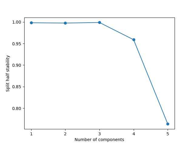
As we can see, there is a sharp drop in stability when increasing from four to five components. This drop indicates that the patterns we find with a five-component model are not robust to small changes in the data. In this case, this result is expected because we simulated the data and know that it contains only four components. So to fit a five-component model to this four-component data, the model might split the information in one of the “true” components into two or more model components and possibly mix some of the components. Since this splitting and mixing can be done in many ways, we no longer have a stable decomposition, causing the sharp drop we see in the plot.
So we see that visualising the split-half stability can be a helpful way to evaluate how many components you should use to model your data.
Split-half analysis for the bike sharing data
Here, we try split-half analysis on bike sharing data from Oslo. This dataset has five modes:
End station
Year
Month
Day of week
Hour of day
The dataset covers all bike trips during 2020 and 2021, and we would expect to find appoximately the same patterns for the two years. We can therefore form two new tensors, one for 2020 and one for 2021, fit PARAFAC models for these two datasets and compare the similarity of the components.
bike_data = tlviz.data.load_oslo_city_bike()
splits = [
bike_data.loc[{"Year": 2020}],
bike_data.loc[{"Year": 2021}],
]
bike_models = {}
for rank in [1, 2, 3, 4, 5]:
print(f"{rank} components")
bike_models[rank] = []
for split in splits:
current_models = fit_many_parafac(split.data, rank)
current_model = tlviz.multimodel_evaluation.get_model_with_lowest_error(current_models, split)
bike_models[rank].append(current_model)
bike_stability = {}
for rank, (cp_1, cp_2) in bike_models.items():
fms = tlviz.factor_tools.factor_match_score(cp_1, cp_2, consider_weights=False, skip_mode=1)
bike_stability[rank] = fms
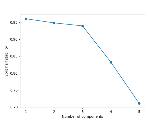
fig, ax = plt.subplots()
ax.plot(bike_stability.keys(), bike_stability.values(), "-o")
ax.set_xticks(list(split_half_stability.keys()))
ax.set_xlabel("Number of components")
ax.set_ylabel("Split half stability")
plt.show()
1 components
2 components
3 components
4 components
5 components
Based on this split-half analysis, we see that we find three components that are present in both years. The moment we go up to four components, the stability drastically falls, and it falls even further with five components. This indicates that three components is a good choice for the model.
Total running time of the script: ( 2 minutes 54.338 seconds)