Note
Click here to download the full example code
Core consistency
A popular metric for evaluating the validity of PARAFAC models is the core consistency diagnostic (sometimes called CORCONDIA) [BK03]. In this example, we’ll see how, why and when the core consistency works well.
We start by fitting a four-component model to the amino acids dataset. First, we import the relevant modules and create a utility function to fit many PARAFAC models.
import matplotlib.pyplot as plt
from tensorly.decomposition import parafac

import tlviz


def fit_parafac(X, num_components, num_inits=5):
    model_candidates = [
        parafac(
            X,
            num_components,
            n_iter_max=1000,
            tol=1e-8,
            init="random",
            orthogonalise=True,
            linesearch=True,
            random_state=i,
        )
        for i in range(num_inits)
    ]
    cp_tensor = tlviz.multimodel_evaluation.get_model_with_lowest_error(model_candidates, X)
    return tlviz.postprocessing.postprocess(cp_tensor, dataset=aminoacids)
Then we load the data and fit a PARAFAC model to it.
aminoacids = tlviz.data.load_aminoacids()
four_component_cp = fit_parafac(aminoacids.data, 4, num_inits=5)
Loading Aminoacids dataset from:
Bro, R, PARAFAC: Tutorial and applications, Chemometrics and Intelligent Laboratory Systems, 1997, 38, 149-171
Now, we want to check the validity of this model. We know that with PARAFAC, we cannot have any interactions between the components. Mathematically this means that our tensor entries, \(x_{ijk}\) is described by
where \(a_{ir},b_{jr}\) and \(c_{kr}\) are entries in the factor matrices, \(\mathbf{A}, \mathbf{B}\) and \(\mathbf{C}\), respectively (we keep the weight multiplied into the factor matrices).
If we want to allow for interactions between our components, we could use a Tucker model. This model introduces linear interactions and represents a tensor by
where \(\mathbf{g}_{r_0 r_1 r_2}\) is an entry in the \(R \times R \times R\) core array. We see that the PARAFAC model is a special case of the Tucker model, where the superdiagonal entries are equal to \(1\) and the off-diagonal entries are equal to \(0\) (\(\mathbf{g}_{r_0 r_1 r_2} = 1\) if \(r_0 = r_1 = r_2\) and \(0\) otherwise). We denote this special core tensor by \(\mathcal{T}\).
We know that if our dataset follows the PARAFAC model and if we have recovered the correct components, we will not get a better fit by allowing for interactions between the components. To check this, we can compute and inspect the optimal \(\mathcal{G}\) given the factor matrices we found with PARAFAC.
Let’s look at the entries we get for \(\mathcal{G}\) with the PARAFAC model we fitted to the amino acids dataset.
tlviz.visualisation.core_element_heatmap(four_component_cp, aminoacids)
plt.show()
![core_tensor[0, :, :], core_tensor[1, :, :], core_tensor[2, :, :], core_tensor[3, :, :]](../_images/sphx_glr_plot_core_consistency_001.png)
This plot shows interaction between the different components. For example, we see that there are high values in the four corners of slab 0 and 3, which indicates a strong two-component interaction between component 3 and component 1. There are also high values in the four corners of slab 1, which shows that there is a three-component interaction between component 0, 1 and 3.
A downside with the core element heatmap is that we can only create it for third-order tensors. Also, while the heatmap shows where the interactions are, it can be difficult to see exactly how strong they are. It is, therefore, also helpful to look at a plot of the core elements, sorted, so the superdiagonal are plotted first, and the off-diagonal entries are plotted afterwards.
tlviz.visualisation.core_element_plot(four_component_cp, aminoacids)
plt.show()
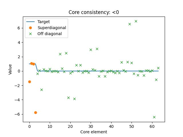
Here, we also see that the core tensor is not similar to \(\mathcal{T}\) (which is plotted with the straight line). Therefore, we can conclude that the amino acids dataset likely does not follow a 4-component PARAFAC model.
To understand why this works, we can consider a noisy dataset that follows an \(R\)-component PARAFAC model. If we fit an \(R\)-component model to this data, we should find the components, and there will be no interaction between them. However, if we fit an \(R+1\)-component model to this data, we will get an extra component that models the noise. This additional component is forced to be trilinear with no interaction, but the process it describes (the noise) is not trilinear. Therefore, this model can better describe the noise by adding interactions with the other modes.
It is common to summarise the above analysis into a single metric by computing the relative difference between \(\mathcal{G}\) and \(\mathcal{T}\). This metric is called the core consistency diagnostic (sometimes called CORCONDIA), and is defined as
A core consistency of 100 signifies that no linear interactions can improve the fit, while a low core consistency indicates that we can improve the fit by including linear interactions (sometimes, the core consistency is defined by dividing by \(\| \mathcal{G} \|^2\) instead of R). We can use the core consistency to select an appropriate PARAFAC model from a set of candidates. Below is an example where we have done that
models = {}
for rank in [1, 2, 3, 4, 5]:
    models[rank] = fit_parafac(aminoacids.data, rank, num_inits=5)

ax = tlviz.visualisation.scree_plot(models, aminoacids, metric="Core consistency")
ax.set_ylim(0, 105)
plt.show()
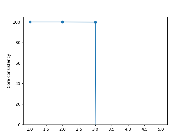
Here, we see that for one, two and three components, the core consistency is high, but when we look at four components, the core consistency becomes very small. The three-component model is, therefore, a good choice.
tlviz.visualisation.core_element_heatmap(models[3], aminoacids)
plt.show()
![core_tensor[0, :, :], core_tensor[1, :, :], core_tensor[2, :, :]](../_images/sphx_glr_plot_core_consistency_004.png)
tlviz.visualisation.core_element_plot(models[3], aminoacids)
plt.show()
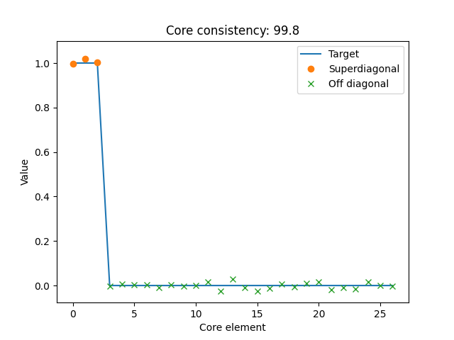
Here, we see that \(\mathcal{G}\) and \(\mathcal{T}\) are very similar, which indicates that the three-component model could be a good choice for this dataset.
Final note
It is important to note that the core consistency is not guaranteed to tell us which model to use. There are several cases where the core consistency may fail. Some examples are:
If we have many components, then even minor differences on the off-diagonal can sum up and reduce the core consistency measurably,
if we have data that doesn’t follow the assumptions of PARAFAC but where the PARAFAC components can still provide valuable insight,
if we need a component to model structural noise to correctly recover the meaningful components.
or if the data is very noisy, the model can potentially improve the fit by allowing for interactions even if we know the true underlying factor matrices.
The core consistency can be very low in all these cases, even for the “best” model. Therefore, it is essential to consider more than just the core consistency when selecting the best model. Examples are initialisation stability, split half stability, and looking at the component vectors to see if they make sense.
Total running time of the script: ( 0 minutes 14.948 seconds)