Optimisation diagnostics with PARAFAC models¶

Fitting PARAFAC models entails solving a non-convex optimisation problem. To do this, we use alternating least squares, (ALS). However, ALS is not guaranteed to converge to the global minimum. It is therefore often advised to use several random initialisations and pick the one that obtained the lowest loss value.

Now, a logical question is, how can we be sure that the decomposition we ended up with is good? There is, unfortunately, no easy answer to this question. But, if we inspect the runs, we can become more confident in our results.

We start by importing the relevant code.

import matplotlib.pyplot as plt
import numpy as np
from tensorly.decomposition import parafac

import tlviz
from tlviz.factor_tools import factor_match_score
from tlviz.multimodel_evaluation import (
    get_model_with_lowest_error,
    similarity_evaluation,
)

Then we create a simulated dataset

rank = 5
cp_tensor, X = tlviz.data.simulated_random_cp_tensor((10, 15, 20), rank, noise_level=0.05, seed=1)

Next, we fit ten random initialisations to this dataset, storing the CP tensors and relative SSE.

estimated_cp_tensors = []
errors = []
for init in range(10):
    print(init)
    est_cp, rec_errors = parafac(X, rank, n_iter_max=100, init="random", return_errors=True, random_state=init)
    estimated_cp_tensors.append(est_cp)
    errors.append(np.array(rec_errors) ** 2)  # rec_errors is relative norm error, we want relative SSE

And get the initialisation

first_attempt = get_model_with_lowest_error(estimated_cp_tensors, X)

To see if we have a good initialisation, we use the optimisation diagnostics plots,

tlviz.visualisation.optimisation_diagnostic_plots(errors, n_iter_max=100)
plt.show()

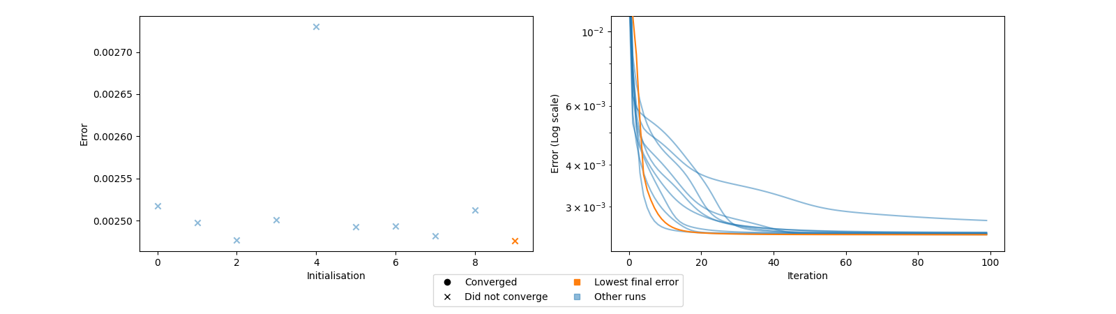
These plots show the final loss value for each initialisation, with markers that signify if the different initialisations converged and the loss plot for each initialisation. We want reproducible results, so ideally, many of the initialisations should achieve the same low loss value. We also want the initialisations to converge.

In this case, we see that we get many different loss values, and they did not converge. These observations indicate that our optimisation procedure did not converge to a good minimum. Another thing we can look at is how similar the different initialisations are with the selected initialisation.

print(similarity_evaluation(first_attempt, estimated_cp_tensors))

[0.4708859077815945, 0.5920264839416483, 0.7423143022576746, 0.5533437244459345, 0.4101864771364167, 0.6463514554345984, 0.588523605705918, 0.6133154419764746, 0.4110835038964634, 1.0]

We see that the different initialisations do not resemble the selected initialisation much. So the optimisation seems unstable. Let’s also compare the selected model with the true decomposition (which is only possible because we have simulated data and therefore know the true decomposition).

print(factor_match_score(first_attempt, cp_tensor))

0.6612200819031797

So the decomposition is, as we expected, not very good… Let’s try to increase the maximum number of iterations!

estimated_cp_tensors = []
errors = []
final_errors = []
for init in range(10):
    print(init)
    est_cp, rec_errors = parafac(X, rank, n_iter_max=1000, init="random", return_errors=True, random_state=init)
    estimated_cp_tensors.append(est_cp)
    errors.append(np.array(rec_errors) ** 2)  # rec_errors is relative norm error, we want relative SSE
second_attempt = get_model_with_lowest_error(estimated_cp_tensors, X)

And plot the optimisation diagnostics plot

tlviz.visualisation.optimisation_diagnostic_plots(errors, 1000)
plt.show()

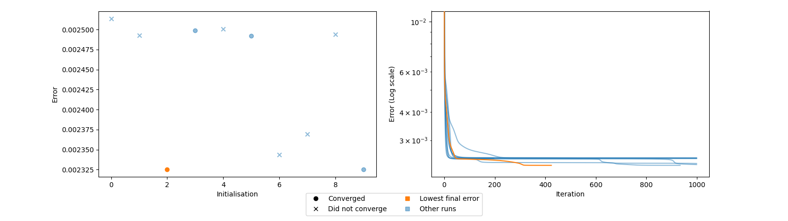
At least some converged, and a couple reached the same loss value. These results are better but not ideal. We don’t want it to be challenging to find a good initialisation! Let’s compare the similarity between the different initialisations and the selected initialisation.

print(similarity_evaluation(second_attempt, estimated_cp_tensors))

[0.5126378280855426, 0.6068598338965694, 1.0, 0.4978209914214167, 0.48813790247489397, 0.6744315207762925, 0.7619003379205388, 0.808697556273191, 0.5034024525852446, 0.9914718665026425]

Ok, we got two similar decompositions. Not ideal, but at least there was more than one good initialisation. Let’s try some more initialisations before we compare with the true decomposition.

for init in range(10, 20):
    print(init)
    est_cp, rec_errors = parafac(X, rank, n_iter_max=1000, init="random", return_errors=True, random_state=init)
    estimated_cp_tensors.append(est_cp)
    errors.append(np.array(rec_errors) ** 2)  # rec_errors is relative norm error, we want relative SSE
third_attempt = tlviz.multimodel_evaluation.get_model_with_lowest_error(estimated_cp_tensors, X)

And let’s look at the optimisation diagnostics plot

tlviz.visualisation.optimisation_diagnostic_plots(errors, 1000)
plt.show()

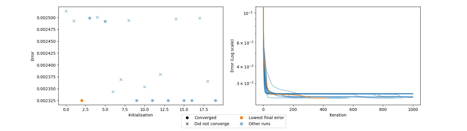
Now we have many initialisations that converged to the same loss value! That is exactly the behaviour that we want. Let’s compare the similarity between them and the selected decomposition too.

print(similarity_evaluation(third_attempt, estimated_cp_tensors))

[0.5126378280855426, 0.6068598338965694, 1.0, 0.4978209914214167, 0.48813790247489397, 0.6744315207762925, 0.7619003379205388, 0.808697556273191, 0.5034024525852446, 0.9914718665026425, 0.8190088546105547, 0.9775165519844442, 0.7283332135990132, 0.9907696759770579, 0.6357626037558478, 0.9775611091933538, 0.9912200986979351, 0.5736136740755231, 0.7574342297346058, 0.9889962033747681]

Here we also see that many of the initialisations were similar. If these were different, we would be in trouble. Since then, there would likely be many different minima with the same loss value. Luckily, that was not the case. Finally, let’s compare our selected model with the true decomposition!

print(factor_match_score(cp_tensor, third_attempt))

decompositions = {
    "True": cp_tensor,
    "First attempt": first_attempt,
    "Second attempt": second_attempt,
    "Third attempt": third_attempt,
}
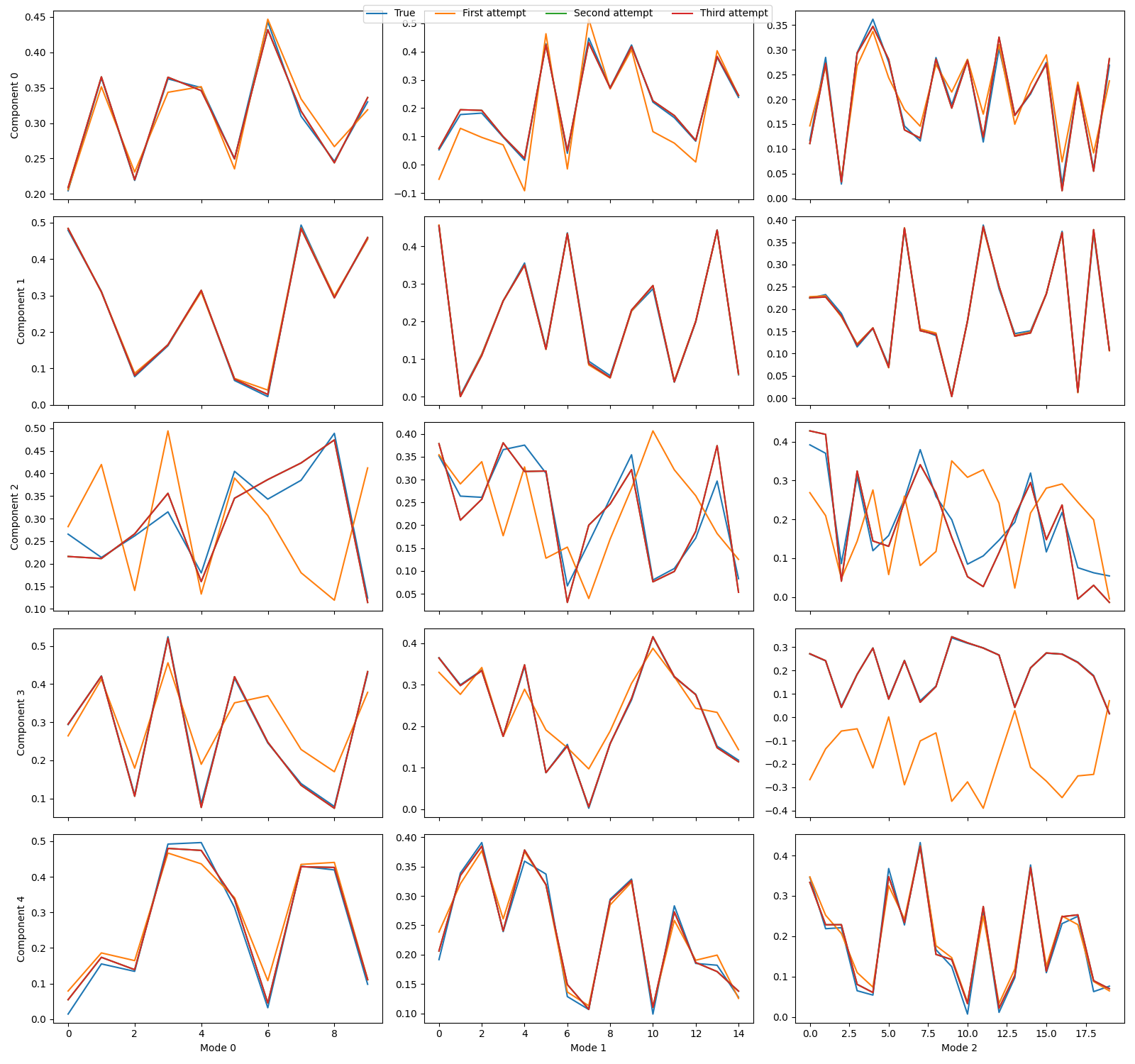
tlviz.visualisation.component_comparison_plot(decompositions, row="component")
plt.show()

0.9321826461235213

Total running time of the script: ( 0 minutes 17.961 seconds)

Gallery generated by Sphinx-Gallery