Selecting the number of components in PARAFAC models¶

Imports and utilities¶

import matplotlib.pyplot as plt
from tensorly.decomposition import parafac

import tlviz

To fit PARAFAC models, we need to solve a non-convex optimization problem, possibly with local minima. It is therefore useful to fit several models with the same number of components using many different random initialisations.

def fit_many_parafac(X, num_components, num_inits=5):
    return [
        parafac(
            X,
            num_components,
            n_iter_max=1000,
            tol=1e-8,
            init="random",
            orthogonalise=True,
            linesearch=True,
            random_state=i,
        )
        for i in range(num_inits)
    ]

Loading the data¶

Here we load the Aminoacids dataset from [Bro97] and plot the EEM-matrix for each of the five samples.

aminoacids = tlviz.data.load_aminoacids()

fig, axes = plt.subplots(1, 5, figsize=(15, 3), tight_layout=True)
for i, sample in enumerate(aminoacids):
    sample.plot(ax=axes[i], vmin=0, vmax=600)

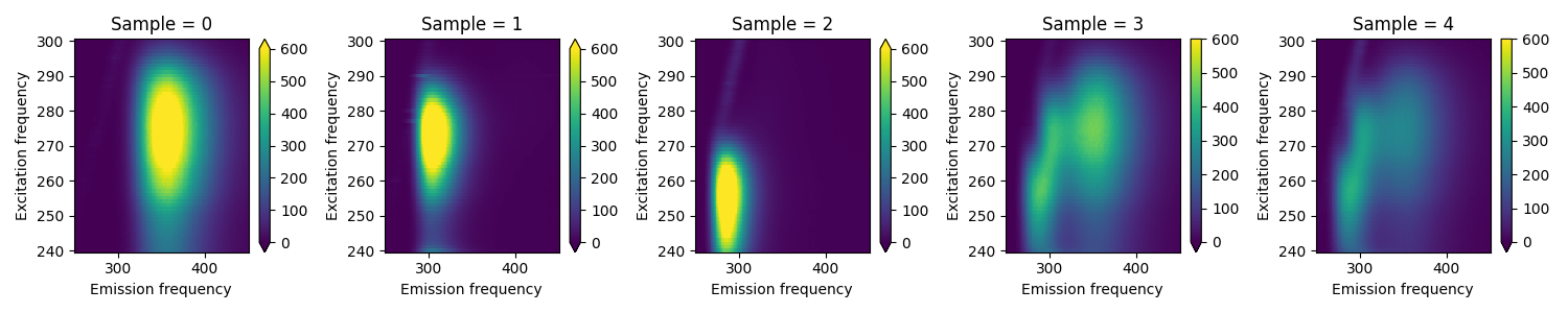
Loading Aminoacids dataset from:
Bro, R, PARAFAC: Tutorial and applications, Chemometrics and Intelligent Laboratory Systems, 1997, 38, 149-171

Fit models¶

models = {}
for rank in [1, 2, 3, 4, 5]:
    print(f"{rank} components")
    models[rank] = fit_many_parafac(aminoacids.data, rank, num_inits=5)

1 components
2 components
3 components
4 components
5 components

Sort the initialisation by their SSE¶

For each rank, we pick the initialization that achieved the lowest reconstruction error. To do this, we first sort each initialization by its final relative sum squared error (rel. SSE).

errors = {}
for rank, inits in models.items():
    sorted_inits, sorted_errors = tlviz.multimodel_evaluation.sort_models_by_error(inits, aminoacids.data)
    models[rank] = sorted_inits
    errors[rank] = sorted_errors

selected_models = {rank: inits[0] for rank, inits in models.items()}

Examine model uniqueness¶

To examine whether we have found the global minimum, we compare each initialization with the initialization that achieved the lowest rel. SSE. Ideally, we want the initializations to have reached the same point, and if that is the case, they should have the same rel. SSE and similar components. To measure the component similarity, we use the factor match score (FMS), similar to the cosine similarity score. An FMS value of 1 indicates that the components are equivalent. The FMS is given by

where the the parameters without a hat correspond the the parameters of the reference decomposition. \(w\) represents the weight of the decompositions, and \(\mathbf{a}_r, \mathbf{b}_r\) and \(\mathbf{c}_r\) represents the \(r\)-th component vectors.

fms_with_selected = {}
for rank, inits in models.items():
    fms_with_selected[rank] = tlviz.multimodel_evaluation.similarity_evaluation(inits[0], inits)

Plot uniqueness information¶

A visual way to examine the uniqueness is to plot the rel. SSE on one axis and the FMS with selected initialization on the other axis for each initialization. We create one such plot for each rank to compare different choices of rank

fig, axes = plt.subplots(1, 5, figsize=(15, 3), tight_layout=True, sharex=True, sharey=True)

for i, rank in enumerate(errors):
    axes[i].scatter(fms_with_selected[rank], errors[rank], alpha=0.8)
    axes[i].set_title(f"{rank} components")
    axes[i].set_xlabel("FMS with best")
    axes[i].set_yscale("log")

axes[0].set_ylabel("Relative SSE")
plt.show()

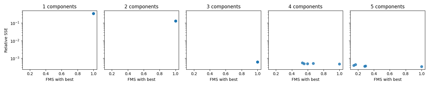
From this plot, we see that for 1-3 components, all initializations seem to achieve the same rel. SSE and similar components. This similarity indicates that the models are unique. However, for 4-5 components, we see that the “FMS with best” value is low, which means that the selected initialization is quite different from the rest. This difference indicates that we either have a non-unique model or problems with local minima. Therefore, if we decide to go with the four or five component models, we should run even more initializations to ensure that we can get the same components for more than just one initialization.

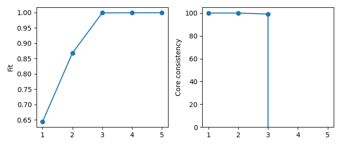
Scree plot of fit and core consistency¶

Another common strategy for determining the number of components is the fit and core consistency diagnostic. The fit measures how well the model describes the data. By plotting this value for each rank choice, we can see how much additional components improve the model fit. We are looking for a “shoulder” where the fit increase slows down, indicating that the added complexity of a higher rank model does not actually add much in terms of modelling the data.

The core consistency measure “interaction” between the components of the model. The PARAFAC model assumes multi-linearity, which means that the components don’t interact, and the uniqueness of PARAFAC stems from this assumption. A low core consistency value means that allowing for component interaction could improve the model’s fit, which indicates that the components are modelling behavior that is not multilinear. Therefore, the core consistency can be a good metric for selecting the number of components as a drop in core consistency can indicate that you have added too many components and started modelling noise or patterns that do not satisfy the multilinearity assumption of PARAFAC. However, the PARAFAC model can be useful even if the data does not follow the multilinearity assumption. Hence, a low core consistency alone is not necessarily a bad sign.

fig, axes = plt.subplots(1, 2, figsize=(7, 3), tight_layout=True)

tlviz.visualisation.scree_plot(selected_models, aminoacids.data, metric="Fit", ax=axes[0])
tlviz.visualisation.scree_plot(selected_models, aminoacids.data, metric="Core consistency", ax=axes[1])

axes[1].set_ylim(0, 105)
plt.show()

Core element plot¶

The core element plot shows the elements of the core tensor. Ideally “Superdiagonal” entries should be 1 and off-diagonal entries should be zero which means no interaction.

One thing to note is that as the number of components increases, so does the number of possible interactions. So models with a high number of components are more likely to be improved by allowing interactions than models with a low number of components. Thus, the core consistency is a less precise metric if you expect your data needs a high number of components.

fig, axes = plt.subplots(1, 5, figsize=(15, 3), tight_layout=True, sharex=False, sharey=False)

for i, (rank, model) in enumerate(selected_models.items()):
    axes[i].set_title(f"{rank} components")
    tlviz.visualisation.core_element_plot(model, aminoacids.data, ax=axes[i])

plt.show()

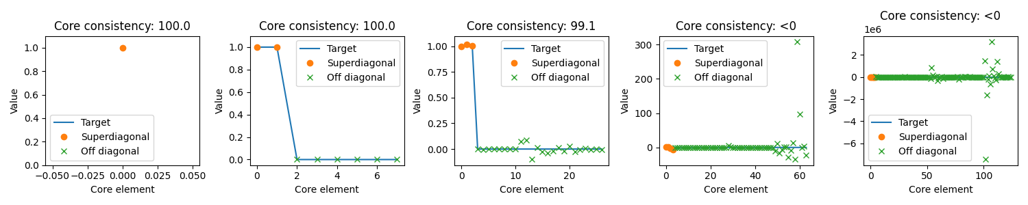
For more information about the core consistency and core element plot, see the core consistency example.

Split-half analysis¶

Another way to select the number of components is with split-half analysis. With split-half analysis, we divide the dataset in two along one mode, and fit two different models, one for each split. Then, we compare the similarity of the decomposition for the modes where we did not perform the split.

For split-half analysis, it is important to choose a split that makes sense. We need to expect that all components will be present in both splits! In this case, we only have five samples, and reducing the number of samples even further can make it difficult to find the correct decomposition. We will therefore not use split-half analysis here. Instead, we have devoted a separate example for split-half analysis.

Component plots¶

When deciding the number of components, the most important consideration is the components themselves. It is therefore essential to visualize the components and evaluate whether they are meaningful in terms of the application

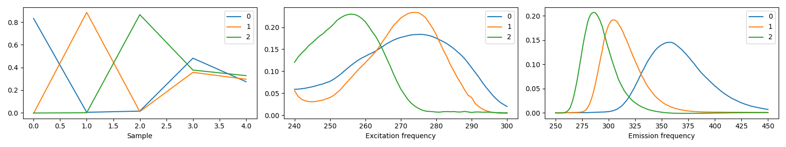
3 components¶

model_3comp = tlviz.postprocessing.postprocess(selected_models[3], dataset=aminoacids)
tlviz.visualisation.components_plot(model_3comp)
plt.show()

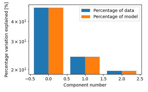
fig, ax = plt.subplots(figsize=(3 * 1.6, 3), tight_layout=True)
tlviz.visualisation.percentage_variation_plot(model_3comp, aminoacids.data, method="both", ax=ax)
ax.set_yscale("log")
plt.show()

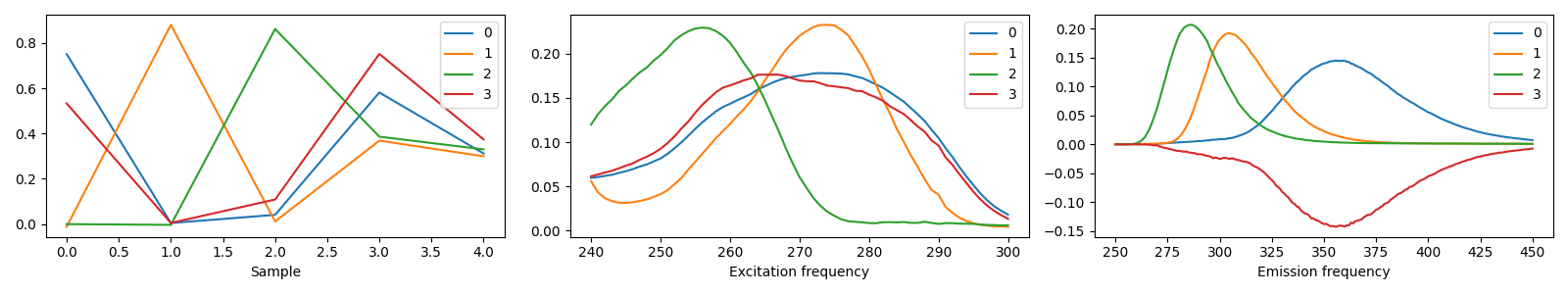
4 components¶

model_4comp = tlviz.postprocessing.postprocess(selected_models[4], dataset=aminoacids)
tlviz.visualisation.components_plot(model_4comp)
plt.show()

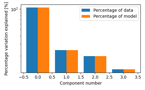
fig, ax = plt.subplots(figsize=(3 * 1.6, 3), tight_layout=True)
tlviz.visualisation.percentage_variation_plot(model_4comp, aminoacids.data, method="both", ax=ax)
ax.set_yscale("log")

We see that the three-component model consists of three clear chemical spectra, which coincides well with our knowledge of the data. The data contains five samples, and each sample represents the emission excitation matrix of a mixture of three aminoacids. The sample-mode component shows the concentration of each chemical, and the emission- and excitation-mode components show the emission- and excitation-spectra of the chemicals (all in arbitrary units). With more than three components, we find that one of the components has negative, and therefore unphysical, values.

Total running time of the script: ( 0 minutes 15.056 seconds)

Download Python source code: plot_selecting_aminoacids_components.py

Download Jupyter notebook: plot_selecting_aminoacids_components.ipynb

Gallery generated by Sphinx-Gallery