Note
Go to the end to download the full example code.
Outlier detection with PARAFAC
There are two metrics that are commonly used for detecting outliers in PARAFAC models: leverage and residuals.
Residuals
The residuals measure how well the PARAFAC model represents the data. For detecting outliers, it is common to compute the sum of squared error for each sample. Since each sample corresponds to a slab in the data tensor, we use the name slabwise SSE in TLViz. For a third-order tensor, \(\mathcal{X}\), and its PARAFAC estimate, \(\hat{\mathcal{X}}\), we compute the \(i\)-th residual in the first mode as
These residuals measure how well our decomposition fits the different samples. If a sample, \(i\), has a high residual, then that indicates that our PARAFAC model cannot describe its behaviour.
Leverage
The leverage score measures how “influential” the different samples are for the PARAFAC model. There are several interpretations of the leverage score [VW81], one of them is the number of components we devote to a given data point. To compute the leverage score for the different samples, we only need the factor matrix for the sample mode. If the sample mode is represented by \(\mathbf{A}\), then the leverage score is defined as
that is, the \(i\)-th diagonal entry of the matrix \(\mathbf{A} \left(\mathbf{A}^T \mathbf{A}\right)^{-1} \mathbf{A}^T\).
Examples with code
Below, we show some examples with simulated data to illustrate how we can use the leverage and residuals to find and remove the outliers in a dataset.
import matplotlib.pyplot as plt
import numpy as np
import pandas as pd
from tensorly.decomposition import parafac

import tlviz
Utility for fitting PARAFAC models and sampling CP tensors
def fit_parafac(X, num_components, num_inits=5):
    model_candidates = [
        parafac(
            X.data,
            num_components,
            n_iter_max=1000,
            tol=1e-8,
            init="random",
            orthogonalise=True,
            linesearch=True,
            random_state=i,
        )
        for i in range(num_inits)
    ]
    model = tlviz.multimodel_evaluation.get_model_with_lowest_error(model_candidates, X)
    return tlviz.postprocessing.postprocess(model, X)


def index_cp_tensor(cp_tensor, indices, mode):
    weights, factors = cp_tensor
    indices = set(indices)
    new_factors = []
    for i, fm in enumerate(factors):
        if i == mode:
            new_factors.append(fm[fm.index.isin(indices)])
        else:
            new_factors.append(fm)

    return weights, new_factors
Generate simulated dataset
We start by generating a random CP Tensor where the first mode represents the sample mode, and the other two modes represent some signal we have measured.
I, J, K = 20, 30, 40
rank = 5
offset = np.arange(1, rank + 1)[np.newaxis]

rng = np.random.default_rng(0)
A = pd.DataFrame(rng.standard_normal((I, rank)))
A.index.name = "Mode 0"
B = pd.DataFrame(np.sin(offset * np.linspace(0, 2 * np.pi, J)[:, np.newaxis] / rank + offset))
B.index.name = "Mode 1"
C = pd.DataFrame(np.cos(offset * np.linspace(0, 2 * np.pi, K)[:, np.newaxis] / rank + offset))
C.index.name = "Mode 2"


true_model = (None, [A, B, C])
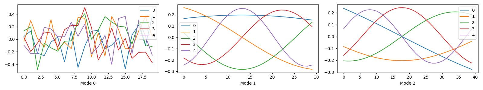
Plotting the components
tlviz.visualisation.components_plot(true_model)
plt.show()
Adding artificial noise
X = tlviz.utils.cp_to_tensor(true_model)
noise = rng.standard_normal(X.shape)
X += np.linalg.norm(X.data) * 0.1 * noise / np.linalg.norm(noise)
Adding artificial outliers
We need three outliers to find; let’s make three of the first four samples into outliers.
X[0] = np.random.standard_normal(X[0].shape)
X[2] *= 10
X[3] = X[3] * 3 + 5
Fitting a PARAFAC model to this data and plotting the components
first_attempt = fit_parafac(X, rank, num_inits=5)
tlviz.visualisation.component_comparison_plot({"True": true_model, "First attempt": first_attempt})
plt.show()
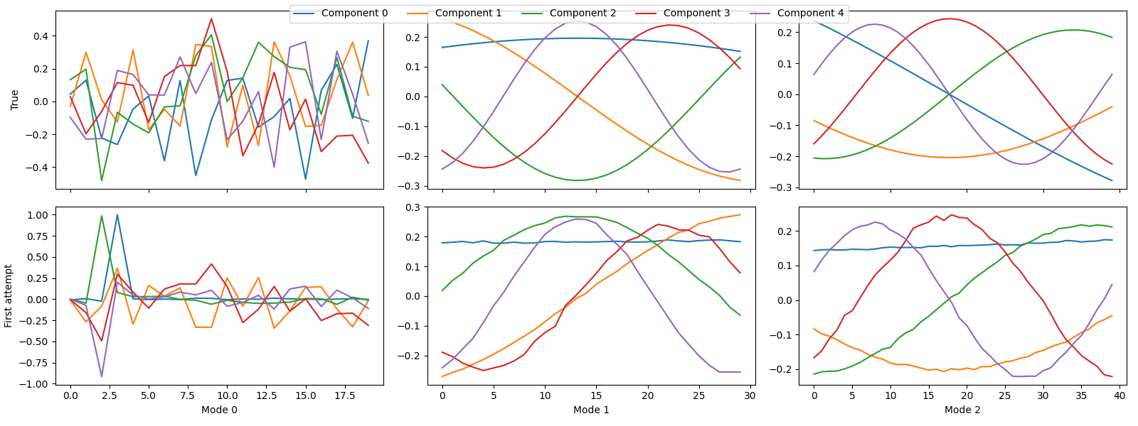
We see that some of the components are wrong, and to quantify this, we can look at the factor match score:
fms = tlviz.factor_tools.factor_match_score(true_model, first_attempt)
print(f"The FMS is {fms:.2f}")
The FMS is 0.39
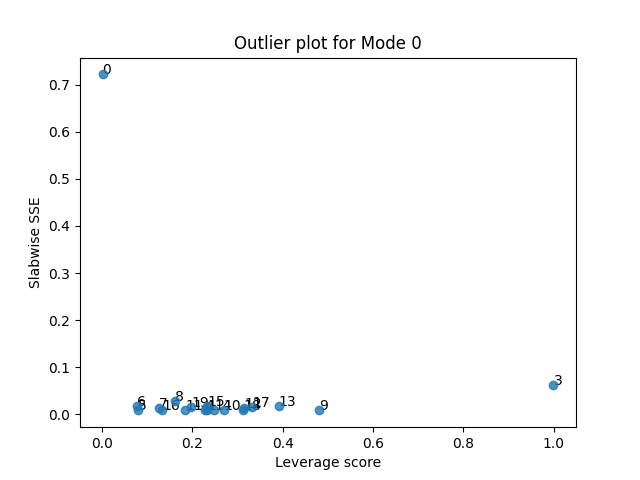
Next, we can create a scatter plot where we plot the leverage and residuals for each sample.
tlviz.visualisation.outlier_plot(first_attempt, X)
plt.show()
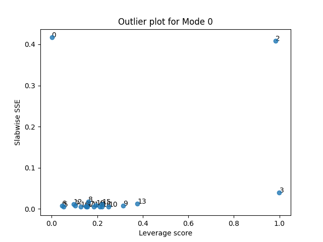
From this plot, we see that there are three potential outliers. First, sample 2 has a high leverage and a high residual. The leverage is close to one, so we almost devote a whole component to modelling it. And still, it is poorly described by the model. We also see that sample 3 has a high leverage and low error, and sample 0 has a low leverage and a high error. Let’s start by removing the most problematic sample: Sample 2.
samples_to_remove = {2}
selected_samples = [i for i in range(I) if i not in samples_to_remove]
sampled_X = X.loc[{"Mode 0": selected_samples}]
second_attempt = fit_parafac(sampled_X, rank, num_inits=5)
Next, we want to compare the true and estimated components. However, since we have removed a slab from the dataset, we also need to remove the corresponding row from \(\mathbf{A}\) before we can compare the components. Otherwise, we could not align the components.
sampled_true_cp = index_cp_tensor(true_model, selected_samples, mode=0)
tlviz.visualisation.component_comparison_plot({"True": sampled_true_cp, "Second attempt": second_attempt})
plt.show()
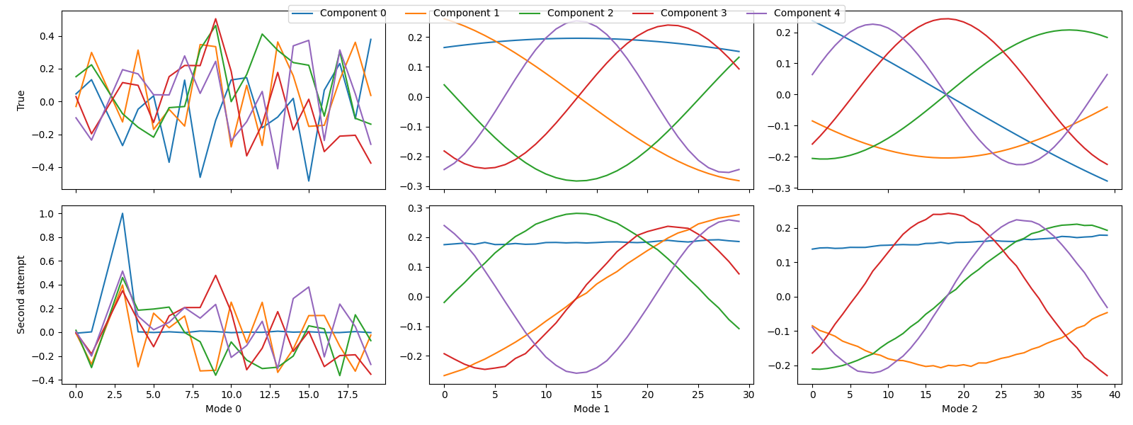
Still, we have not successfully recovered the correct components, which is apparent from the factor match score.
fms = tlviz.factor_tools.factor_match_score(sampled_true_cp, second_attempt)
print(f"The FMS is {fms:.2f}")
The FMS is 0.66
We can also create the outlier plot again to see which samples are suspicious.
tlviz.visualisation.outlier_plot(second_attempt, sampled_X)
plt.show()
We see that sample 0 and 3 still show the same behaviour as before. Sample 0 has a high error, but does not affect the model much, while sample 3 has a low error, but does affect the model. Let us therefore remove sample 3 now.
samples_to_remove = {2, 3}
selected_samples = [i for i in range(I) if i not in samples_to_remove]
sampled_X = X.loc[{"Mode 0": selected_samples}]
third_attempt = fit_parafac(sampled_X, rank, num_inits=5)

sampled_true_cp = index_cp_tensor(true_model, selected_samples, mode=0)
tlviz.visualisation.component_comparison_plot({"True": sampled_true_cp, "Third attempt": third_attempt})
plt.show()
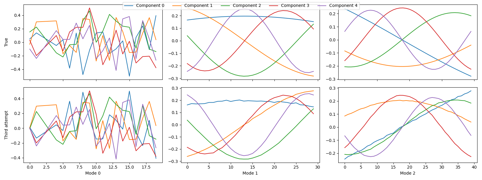
Here, we see that we finally uncovered the true components. This is also apparent from the FMS
fms = tlviz.factor_tools.factor_match_score(sampled_true_cp, third_attempt)
print(f"The FMS is {fms:.2f}")
The FMS is 0.96
Note
Here, we remove the outlier with a very high leverage. However, sometimes, it is better to include the samples with a high leverage and low residual and increase the number of components. Then the additional components can model the samples with the high leverage scores. In this example, we could have increased the number of components by one and recovered the correct components without removing this sample.
We can also create the outlier plot again to see if there still are any suspicious samples
tlviz.visualisation.outlier_plot(third_attempt, sampled_X)
plt.show()
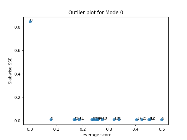
Let’s see what happens when we also remove the final suspicious sample
samples_to_remove = {0, 2, 3}
selected_samples = [i for i in range(I) if i not in samples_to_remove]
sampled_X = X.loc[{"Mode 0": selected_samples}]
fourth_attempt = fit_parafac(sampled_X, rank, num_inits=5)

sampled_true_cp = index_cp_tensor(true_model, selected_samples, mode=0)
tlviz.visualisation.component_comparison_plot({"True": sampled_true_cp, "Fourth attempt": fourth_attempt})
plt.show()
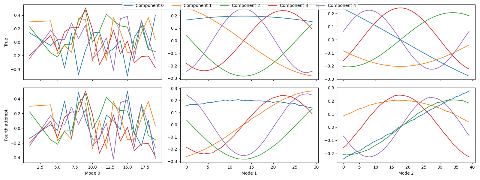
The components didn’t change much.
We didn’t need to remove the final suspicious outlier in this case, and after removing it, the components didn’t change much. This behaviour makes sense because the sample had a very low leverage, so it didn’t affect the model very much. So, in cases where a data point has high residual but not high leverage, it might be sensible not to remove it.
Rules-of-thumb for selecting the samples that may be outliers
Unfortunately, there are no hard rules for selecting which samples to remove as outliers.
Instead, we generally have to consider each suspected outlier individually.
However, there are some useful rules-of-thumb discussed in the literature.
These methods are detailed in tlviz.outliers.get_slabwise_sse_outlier_threshold()
and tlviz.outliers.get_slabwise_sse_outlier_threshold().
There are two ways to select outliers based on the leverage score.
If we interpret the leverage score as the number of components devoted to each sample,
which Huber does in [HR09],
then it makes sense to use a constant cut-off equal to 0.5
(we devote more than half a component to model a single sample) or 0.2
(we devote 20% of a component for a single sample).
Alternatively, we can assume that the components are normally distributed
and use probability theory to estimate the cut-off values.
This approach is what Hoaglin and Welch use in [BKW80]
to obtain their easy-to-compute thresholds.
Finally, we can compute the thresholds using p-values by assuming that the data
either comes from a normal distribution [BKW80],
or from a zero-mean normal distribution [NM95]
(Hotelling T2 p-values).
For selecting the outliers based on the residuals,
we can either assume that the noise is normally distributed
and compute the cut-off values with p-values via a chi-squared distribution
[NM95],
or we can set the cut-off equal to twice the standard deviation of the SSE [NaesIFD02].
Visualising the rules-of-thumb on our first attempted PARAFAC model
tlviz.visualisation.outlier_plot(
    first_attempt,
    X,
    leverage_rules_of_thumb=["p-value", "hotelling", "huber higher", "huber lower", "hw lower", "hw higher"],
    residual_rules_of_thumb=["p-value", "two sigma"],
)
plt.show()
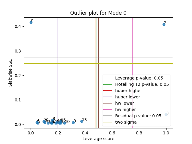
We see that in this case,
all thresholds except "huber lower" successfully detected the outliers.
However, with real data, it is usually not this clear.
Different cut-off values can give different outliers.
Therefore, it is crucial to look at the data and evaluate which data points
to remove and not on a case-by-case basis.
Total running time of the script: (0 minutes 5.004 seconds)