Note
Go to the end to download the full example code.
Non-negative CP decomposition in Tensorly >=0.6
Example and comparison of Non-negative Parafac decompositions.
Introduction
Since version 0.6 in Tensorly, several options are available to compute non-negative CP (NCP), in particular several algorithms:
Multiplicative updates (MU) (already in Tensorly < 0.6)
Non-negative Alternating Least Squares (ALS) using Hierarchical ALS (HALS)
Non-negativity is an important constraint to handle for tensor decompositions. One could expect that factors must have only non-negative values after it is obtained from a non-negative tensor.
import numpy as np
import tensorly as tl
from tensorly.decomposition import non_negative_parafac, non_negative_parafac_hals
from tensorly.decomposition._cp import initialize_cp
from tensorly.cp_tensor import CPTensor
import time
from copy import deepcopy
Create synthetic tensor
There are several ways to create a tensor with non-negative entries in Tensorly. Here we chose to generate a random from the sequence of integers from 1 to 24000.
# Tensor generation
tensor = tl.tensor(np.arange(24000).reshape((30, 40, 20)), dtype=tl.float32)
Our goal here is to produce an approximation of the tensor generated above
which follows a low-rank CP model, with non-negative coefficients. Before
using these algorithms, we can use Tensorly to produce a good initial guess
for our NCP. In fact, in order to compare both algorithmic options in a
fair way, it is a good idea to use same initialized factors in decomposition
algorithms. We make use of the initialize_cp function to initialize the
factors of the NCP (setting the non_negative option to True)
and transform these factors (and factors weights) into
an instance of the CPTensor class:
weights_init, factors_init = initialize_cp(
    tensor, non_negative=True, init="random", rank=10
)

cp_init = CPTensor((weights_init, factors_init))
Non-negative Parafac
From now on, we can use the same cp_init tensor as the initial tensor when
we use decomposition functions. Now let us first use the algorithm based on
Multiplicative Update, which can be called as follows:
tic = time.time()
tensor_mu, errors_mu = non_negative_parafac(
    tensor, rank=10, init=deepcopy(cp_init), return_errors=True
)
cp_reconstruction_mu = tl.cp_to_tensor(tensor_mu)
time_mu = time.time() - tic
Here, we also compute the output tensor from the decomposed factors by using the cp_to_tensor function. The tensor cp_reconstruction_mu is therefore a low-rank non-negative approximation of the input tensor; looking at the first few values of both tensors shows that this is indeed the case but the approximation is quite coarse.
print("reconstructed tensor\n", cp_reconstruction_mu[10:12, 10:12, 10:12], "\n")
print("input data tensor\n", tensor[10:12, 10:12, 10:12])
reconstructed tensor
 [[[8237.63 8286.92]
  [8336.44 8180.15]]

 [[9057.33 9233.85]
  [9068.9  8992.75]]]

input data tensor
 [[[8210. 8211.]
  [8230. 8231.]]

 [[9010. 9011.]
  [9030. 9031.]]]
Non-negative Parafac with HALS
Our second (new) option to compute NCP is the HALS algorithm, which can be used as follows:
tic = time.time()
tensor_hals, errors_hals = non_negative_parafac_hals(
    tensor, rank=10, init=deepcopy(cp_init), return_errors=True
)
cp_reconstruction_hals = tl.cp_to_tensor(tensor_hals)
time_hals = time.time() - tic
Again, we can look at the reconstructed tensor entries.
print("reconstructed tensor\n", cp_reconstruction_hals[10:12, 10:12, 10:12], "\n")
print("input data tensor\n", tensor[10:12, 10:12, 10:12])
reconstructed tensor
 [[[8210.48 8210.36]
  [8230.42 8230.47]]

 [[9010.47 9010.4 ]
  [9030.41 9030.5 ]]]

input data tensor
 [[[8210. 8211.]
  [8230. 8231.]]

 [[9010. 9011.]
  [9030. 9031.]]]
Non-negative Parafac with Exact HALS
From only looking at a few entries of the reconstructed tensors, we can already see a huge gap between HALS and MU outputs. Additionally, HALS algorithm has an option for exact solution to the non-negative least squares subproblem rather than the faster, approximate solution. Note that the overall HALS algorithm will still provide an approximation of the input data, but will need longer to reach convergence. Exact subroutine solution option can be used simply choosing exact as True in the function:
tic = time.time()
tensorhals_exact, errors_exact = non_negative_parafac_hals(
    tensor, rank=10, init=deepcopy(cp_init), return_errors=True, exact=True
)
cp_reconstruction_exact_hals = tl.cp_to_tensor(tensorhals_exact)
time_exact_hals = time.time() - tic
Comparison
First comparison option is processing time for each algorithm:
print(str(f"{time_mu:.2f}") + " " + "seconds")
print(str(f"{time_hals:.2f}") + " " + "seconds")
print(str(f"{time_exact_hals:.2f}") + " " + "seconds")
0.04 seconds
0.56 seconds
199.95 seconds
As it is expected, the exact solution takes much longer than the approximate solution, while the gain in performance is often void. Therefore we recommend to avoid this option unless it is specifically required by the application. Also note that on appearance, both MU and HALS have similar runtimes. However, a closer look suggest they are indeed behaving quite differently. Computing the error between the output and the input tensor tells that story better. In Tensorly, we provide a function to calculate Root Mean Square Error (RMSE):
from tensorly.metrics.regression import RMSE

print(RMSE(tensor, cp_reconstruction_mu))
print(RMSE(tensor, cp_reconstruction_hals))
print(RMSE(tensor, cp_reconstruction_exact_hals))
220.3588
3.8795087
1.2040633
According to the RMSE results, HALS is better than the multiplicative update with both exact and approximate solution. In particular, HALS converged to a much lower reconstruction error than MU. We can better appreciate the difference in convergence speed on the following error per iteration plot:
import matplotlib.pyplot as plt


def each_iteration(a, b, c, title):
    fig = plt.figure()
    fig.set_size_inches(10, fig.get_figheight(), forward=True)
    plt.plot(a)
    plt.plot(b)
    plt.plot(c)
    plt.title(str(title))
    plt.legend(["MU", "HALS", "Exact HALS"], loc="upper left")


each_iteration(errors_mu, errors_hals, errors_exact, "Error for each iteration")
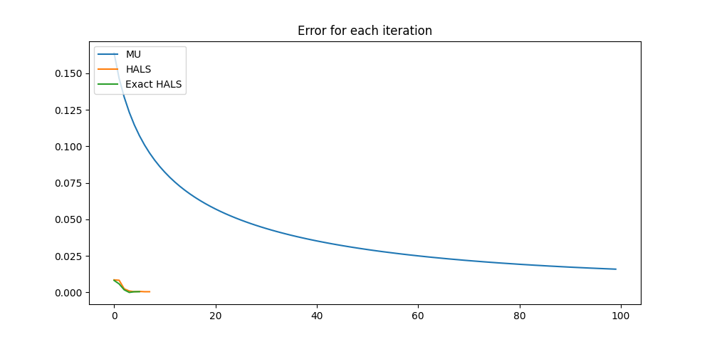
In conclusion, on this quick test, it appears that the HALS algorithm gives much better results than the MU original Tensorly methods. Our recommendation is to use HALS as a default, and only resort to MU in specific cases (only encountered by expert users most likely).
References
Gillis, N., & Glineur, F. (2012). Accelerated multiplicative updates and hierarchical ALS algorithms for nonnegative matrix factorization. Neural computation, 24(4), 1085-1105. (Link) <https://direct.mit.edu/neco/article/24/4/1085/7755/Accelerated-Multiplicative-Updates-and>
Total running time of the script: (3 minutes 20.624 seconds)