Demonstration of PARAFAC2

Example of how to use the PARAFAC2 algorithm.

import numpy as np
import numpy.linalg as la
import matplotlib.pyplot as plt
import tensorly as tl
from tensorly.decomposition import parafac2
from scipy.optimize import linear_sum_assignment

Create synthetic tensor

Here, we create a random tensor that follows the PARAFAC2 constraints found inx (Kiers et al 1999).

This particular tensor, $\mathcal{X} \in \mathbb{R}^{I\times J \times K}$, is a shifted CP tensor, that is, a tensor on the form:

\[\mathcal{X}_{ijk} = \sum_{r=1}^R A_{ir} B_{\sigma_i(j) r} C_{kr},\]

where $\sigma_i$ is a cyclic permutation of $J$ elements.

# Set parameters
true_rank = 3
I, J, K = 30, 40, 20
noise_rate = 0.1
np.random.seed(0)

# Generate random matrices
A_factor_matrix = np.random.uniform(1, 2, size=(I, true_rank))
B_factor_matrix = np.random.uniform(size=(J, true_rank))
C_factor_matrix = np.random.uniform(size=(K, true_rank))

# Normalised factor matrices
A_normalised = A_factor_matrix/la.norm(A_factor_matrix, axis=0)
B_normalised = B_factor_matrix/la.norm(B_factor_matrix, axis=0)
C_normalised = C_factor_matrix/la.norm(C_factor_matrix, axis=0)

# Generate the shifted factor matrix
B_factor_matrices = [np.roll(B_factor_matrix, shift=i, axis=0) for i in range(I)]
Bs_normalised = [np.roll(B_normalised, shift=i, axis=0) for i in range(I)]

# Construct the tensor
tensor = np.einsum('ir,ijr,kr->ijk', A_factor_matrix, B_factor_matrices, C_factor_matrix)

# Add noise
noise = np.random.standard_normal(tensor.shape)
noise /= np.linalg.norm(noise)
noise *= noise_rate*np.linalg.norm(tensor)
tensor += noise

Fit a PARAFAC2 tensor

To avoid local minima, we initialise and fit 10 models and choose the one with the lowest error

best_err = np.inf
decomposition = None

for run in range(10):
    print(f'Training model {run}...')
    trial_decomposition, trial_errs = parafac2(tensor, true_rank, return_errors=True, tol=1e-8, n_iter_max=500, random_state=run)
    print(f'Number of iterations: {len(trial_errs)}')
    print(f'Final error: {trial_errs[-1]}')
    if best_err > trial_errs[-1]:
        best_err = trial_errs[-1]
        err = trial_errs
        decomposition = trial_decomposition
    print('-------------------------------')
print(f'Best model error: {best_err}')

Training model 0...
Number of iterations: 500
Final error: 0.09204720575424472
-------------------------------
Training model 1...
Number of iterations: 500
Final error: 0.09204726856012718
-------------------------------
Training model 2...
Number of iterations: 500
Final error: 0.09269711804187236
-------------------------------
Training model 3...
Number of iterations: 392
Final error: 0.09204692795621944
-------------------------------
Training model 4...
Number of iterations: 415
Final error: 0.09204692959223097
-------------------------------
Training model 5...
Number of iterations: 500
Final error: 0.09291065541285955
-------------------------------
Training model 6...
Number of iterations: 364
Final error: 0.09204692769766268
-------------------------------
Training model 7...
Number of iterations: 424
Final error: 0.09204692883956121
-------------------------------
Training model 8...
Number of iterations: 481
Final error: 0.09204693125447479
-------------------------------
Training model 9...
Number of iterations: 500
Final error: 0.0920563578975846
-------------------------------
Best model error: 0.09204692769766268

A decomposition is a wrapper object for three variables: the weights, the factor matrices and the projection matrices. The weights are similar to the output of a CP decomposition. The factor matrices and projection matrices are somewhat different. For a CP decomposition, we only have the weights and the factor matrices. However, since the PARAFAC2 factor matrices for the second mode is given by

\[B_i = P_i B,\]

where $B$ is an $R \times R$ matrix and $P_i$ is an $I \times R$ projection matrix, we cannot store the factor matrices the same as for a CP decomposition.

Instead, we store the factor matrix along the first mode ($A$), the “blueprint” matrix for the second mode ($B$) and the factor matrix along the third mode ($C$) in one tuple and the projection matrices, $P_i$, in a separate tuple.

If we wish to extract the informative $B_i$ factor matrices, then we use the tensorly.parafac2_tensor.apply_projection_matrices function on the PARAFAC2 tensor instance to get another wrapper object for two variables: weights and factor matrices. However, now, the second element of the factor matrices tuple is now a list of factor matrices, one for each frontal slice of the tensor.

Likewise, if we wish to construct the tensor or the frontal slices, then we can use the tensorly.parafac2_tensor.parafac2_to_tensor function. If the decomposed dataset consisted of uneven-length frontal slices, then we can use the tensorly.parafac2_tensor.parafac2_to_slices function to get a list of frontal slices.

est_tensor = tl.parafac2_tensor.parafac2_to_tensor(decomposition)
est_weights, (est_A, est_B, est_C) = tl.parafac2_tensor.apply_parafac2_projections(decomposition)

Compute performance metrics

reconstruction_error = la.norm(est_tensor - tensor)
recovery_rate = 1 - reconstruction_error/la.norm(tensor)

print(f'{recovery_rate:2.0%} of the data is explained by the model, which is expected with noise rate: {noise_rate}')


# To evaluate how well the original structure is recovered, we calculate the tucker congruence coefficient.

est_A, est_projected_Bs, est_C = tl.parafac2_tensor.apply_parafac2_projections(decomposition)[1]

sign = np.sign(est_A)
est_A = np.abs(est_A)
est_projected_Bs = sign[:, np.newaxis]*est_projected_Bs

est_A_normalised = est_A/la.norm(est_A, axis=0)
est_Bs_normalised = [est_B/la.norm(est_B, axis=0) for est_B in est_projected_Bs]
est_C_normalised = est_C/la.norm(est_C, axis=0)

B_corr = np.array(est_Bs_normalised).reshape(-1, true_rank).T@np.array(Bs_normalised).reshape(-1, true_rank)/len(est_Bs_normalised)
A_corr = est_A_normalised.T@A_normalised
C_corr = est_C_normalised.T@C_normalised

corr = A_corr*B_corr*C_corr
permutation = linear_sum_assignment(-corr)  # Old versions of scipy does not support maximising, from scipy v1.4, you can pass `corr` and `maximize=True` instead of `-corr` to maximise the sum.

congruence_coefficient = np.mean(corr[permutation])
print(f'Average tucker congruence coefficient: {congruence_coefficient}')

91% of the data is explained by the model, which is expected with noise rate: 0.1
Average tucker congruence coefficient: 0.9947046512423608

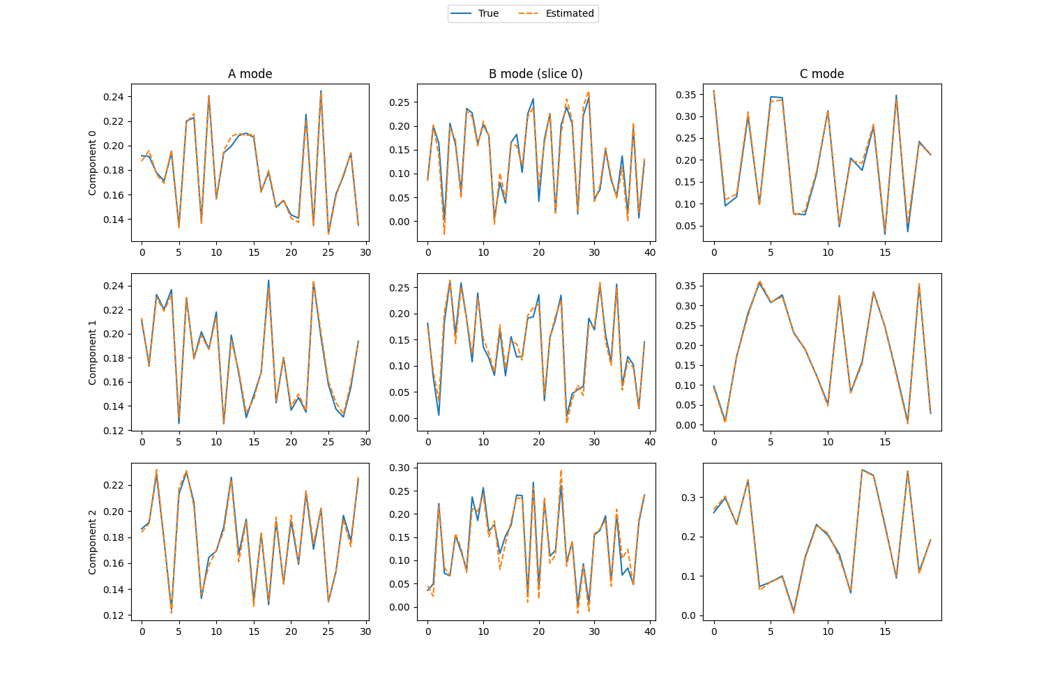
Visualize the components

# Find the best permutation so that we can plot the estimated components on top of the true components
permutation = np.argmax(A_corr*B_corr*C_corr, axis=0)


# Create plots of each component vector for each mode
# (We just look at one of the B_i matrices)

fig, axes = plt.subplots(true_rank, 3, figsize=(15, 3*true_rank+1))
i = 0 # What slice, B_i, we look at for the B mode

for r in range(true_rank):

    # Plot true and estimated components for mode A
    axes[r][0].plot((A_normalised[:, r]), label='True')
    axes[r][0].plot((est_A_normalised[:, permutation[r]]),'--', label='Estimated')

    # Labels for the different components
    axes[r][0].set_ylabel(f'Component {r}')

    # Plot true and estimated components for mode C
    axes[r][2].plot(C_normalised[:, r])
    axes[r][2].plot(est_C_normalised[:, permutation[r]], '--')

    # Plot true components for mode B
    axes[r][1].plot(Bs_normalised[i][:, r])

    # Get the signs so that we can flip the B mode factor matrices
    A_sign = np.sign(est_A_normalised)

    # Plot estimated components for mode B (after sign correction)
    axes[r][1].plot(A_sign[i, r]*est_Bs_normalised[i][:, permutation[r]], '--')

# Titles for the different modes
axes[0][0].set_title('A mode')
axes[0][2].set_title('C mode')
axes[0][1].set_title(f'B mode (slice {i})')

# Create a legend for the entire figure
handles, labels =  axes[r][0].get_legend_handles_labels()
fig.legend(handles, labels, loc='upper center', ncol=2)

<matplotlib.legend.Legend object at 0x7f60dcf476a0>

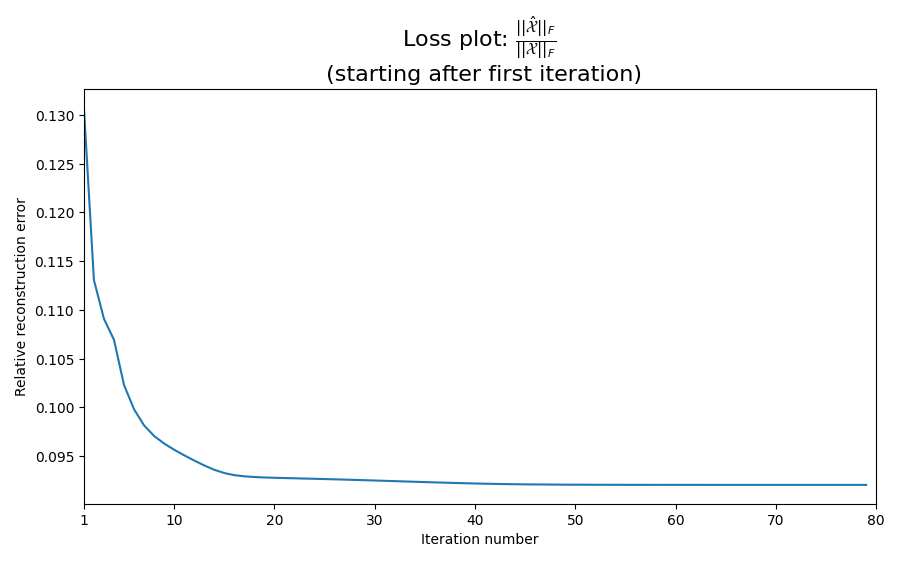
Inspect the convergence rate

It can be interesting to look at the loss plot to make sure that we have converged to a stationary point. We skip the first iteration since the initial loss often dominate the rest of the plot, making it difficult to check for convergence.

loss_fig, loss_ax = plt.subplots(figsize=(9, 9/1.6))
loss_ax.plot(range(1, len(err)), err[1:])
loss_ax.set_xlabel('Iteration number')
loss_ax.set_ylabel('Relative reconstruction error')
mathematical_expression_of_loss = r"$\frac{\left|\left|\hat{\mathcal{X}}\right|\right|_F}{\left|\left|\mathcal{X}\right|\right|_F}$"
loss_ax.set_title(f'Loss plot: {mathematical_expression_of_loss} \n (starting after first iteration)', fontsize=16)
xticks = loss_ax.get_xticks()
loss_ax.set_xticks([1] + list(xticks[1:]))
loss_ax.set_xlim(1, len(err))
plt.tight_layout()
plt.show()

$Loss plot: $\frac{\left|\left|\hat{\mathcal{X}}\right|\right|_F}{\left|\left|\mathcal{X}\right|\right|_F}$ (starting after first iteration)$

References

Kiers HA, Ten Berge JM, Bro R. PARAFAC2—Part I. A direct fitting algorithm for the PARAFAC2 model. Journal of Chemometrics: A Journal of the Chemometrics Society. 1999 May;13(3‐4):275-94. (Online version)

Total running time of the script: ( 0 minutes 34.545 seconds)

Gallery generated by Sphinx-Gallery